
An Intro to Monte Carlo Simulation For Sports Prediction (in Excel)

The growing popularity of sports betting and prediction markets has fueled interest in quantitative methods for assessing event probabilities.
Intro to Monte Carlo Simulations
The Monte Carlo method refers to a statistical technique for predicting uncertain outcomes by running a large number of simulations, each incorporating random variations. This approach allows for the modeling of uncertainty in complex systems, making it valuable for sporting event or election predictions.
Rolling Fair Dice
A basic application of Monte Carlo simulations is estimating the probability of rolling a six on a single throw of a six-sided die through the following steps:
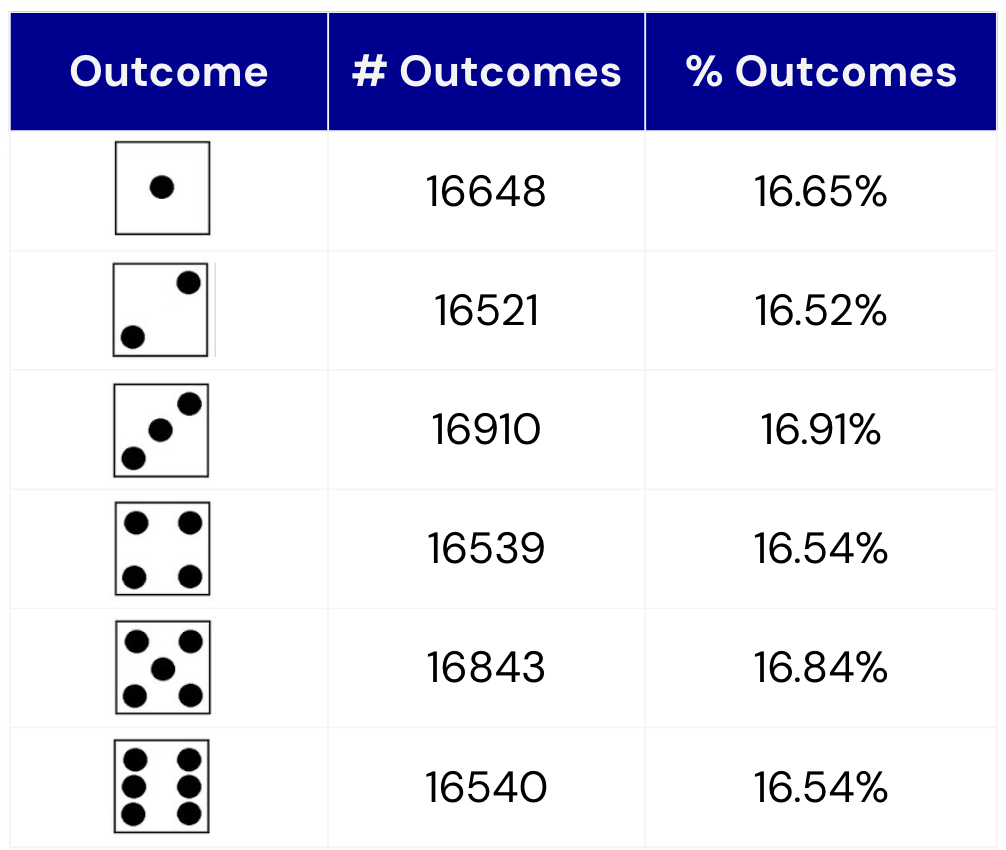
Roll a six-sided die 100,000 times
Tally up each result
Convert the results to frequencies
Use frequencies to predict the distribution of future outcomes
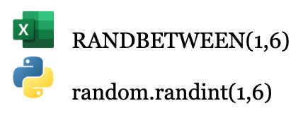
Fortunately, spreadsheets and programming languages make it easy to do this quickly using random number generators.
Rolling Unfair Dice
With minor adjustments, we can also simulate the rolling of non-standard dice.
For example, consider six-sided dice where 4 faces contain blue stickers and 2 faces contain red stickers. How can we use monte carlo simulations to estimate the probability of rolling a blue sticker on a single throw?


We again generate a random number between 1 and 6. If it comes up 1 through 4, we mark that simulation as having resulted in a Blue outcome, otherwise a Red outcome.
Applying Monte Carlo Methods To Sports
It is easy to see how choosing a random number between 1 and 6 “simulates” a six-sided die roll. We can apply this concept to sports using an example matchup between the New Yankees and Boston Red Sox from June 29th, 2019.
The goal is to:
Identify the variables that dictate outcomes (e.g. strength of offense, injuries, home field advantage)
Build a model for the final score of a single game based on those variables
Use the dice rolling technique to simulate remaining uncertainty
Tally results and convert to frequencies
An Example: Yankees vs. Red Sox (June 29, 2019)
Step 1: Identify the variables that dictate outcomes
For a simplified case, we will predict game outcomes by looking at each team’s Average Runs Scored and Average Runs Against.

Step 2: Build a model for the final score of a single game based on those variables
Our model will adjust each team’s expected offensive output based on the quality of the opponent’s defense. When Team A plays Team B, the final score will be:
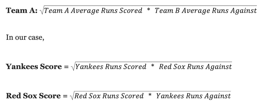

This process yields an expected score of the Yankees beating the Red Sox 5.142 to 4.856. However, it ignores the variability in each team’s performance.
Step 3: Use the dice rolling technique to simulate remaining uncertainty
Even with a simplified model using two variables (Average Runs Scored, Average Runs Against), there is a great deal of uncertainty to be accounted for. This manifests in the standard deviation of each variable.

This is the uncertainty that will be subject to our dice rolling technique. By assuming runs scored are normally distributed (more on that later), we can now utilize the monte carlo method.
To do this, we will use the inverse of the cumulative normal distribution function, which takes 3 parameters in Excel:


We have now “simulated” a matchup between the Yankees and Red Sox in which the Yankees won by a score of 10.147 to 7.945.
However, just as with our dice example, we want to run this simulation not once, but many times:
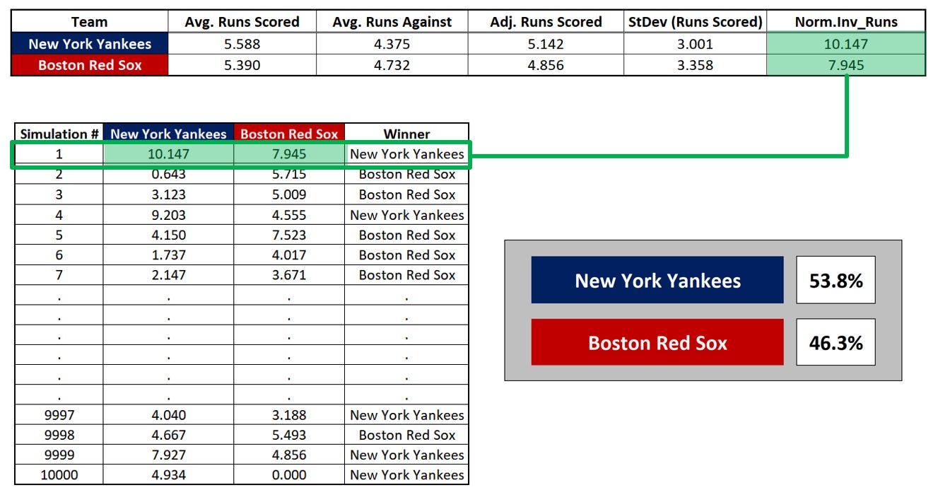
Finally, we can calculate the frequency with which each team won in our simulated matchups and convert or compare those to odds for betting purposes.
Looking Under the Hood
This tactic of first creating a mathematical representation of an event and then iterating through it repeatedly is a standard part of any data scientist’s toolkit and is used to make predictions from weather forecasts to economic data.
We recall from statistics that normally distributed data sets follow a bell curve, under which a specific proportion of values can be found within a given distance from the mean.

Using only the mean and standard deviation of any normal distribution, we can construct a chart like the above. In the context of our model, this chart shows the likelihood with which the Yankees (or a team statistically identical to the Yankees) would score any number of runs against the Red Sox (or a team statistically identical to the Red Sox). Since normal distributions are symmetric about the mean, we would say there is a:
50% chance of scoring up to 5.142 runs
50% + 34.1% = 84.1% of scoring up to 8.143 runs
50% — 34.1% = 15.9% chance of scoring up to 2.141 runs
When building our simulation, we used the inverse of the cumulative normal distribution function along with 3 parameters. The cumulative normal distribution function itself shows, for a given distribution and value of x, the probability of a randomly selected value being less than x. In other words, what percentage of the data falls to the left of x.
In other words, if we choose a value x along the x-axis, this function will tell us the probability that a randomly selected point under the curve will be to the left of that x value.
The inverse of this function does…the inverse. If we supply the mean and standard deviation of a distribution along with a probability z, the NORM.INV function gives us an x value for which z% of data points in that distribution fall to the left.
The percentage or probability that we are supplying, in this case in Excel, comes from a (pseudo) random number generator that outputs a value greater than or equal to 0 and less 1. When the simulation was run to construct these graphics, that random value produced by Excel for the Yankees was ~0.95234.

One interpretation is that, for a bell curve representing a distribution with a mean of 5.142 and standard deviation of 3.001, 95.234% of the values fall to the left of 10.147. Another way of saying this is that the Yankees (or a team statistically identical to the Yankees) will score 10.147 or fewer runs against the Red Sox (or a team statistically identical to the Red Sox) in 95.234% of matchups.
As long as the assumption of a normal distribution holds, iteratively using random values between 0 and 1 to generate simulated scores for each team will give us a good approximation of how the game we parameterized is likely to play out (hopefully). However, for low-scoring sports like soccer and baseball, a Poisson distribution or negative binomial distribution is more appropriate.
In this case it is possible to obtain a negative number of runs scored. For the purposes of the model we are building, we will employ logic that converts any negative scores to a score of 0.000. Perhaps a simulated score of Yankees: -4, Red Sox: -3 is just as informative as a simulated score of Yankees: 5, Red Sox: 6. Or, perhaps one wants to completely remove the entire simulated matchup in the case that either team produces a result that would be impossible in the real world.
This is not the only aspect of our model that leaves room for creativity and also for error. We did not take into account home field advantage, injuries, momentum, weather, stadium dimensions, starting pitchers, and a host of other important data points that may impact our predictions.
Home Field Advantage
During the 2018 MLB regular season the home team won 1,277 games (52.6%), while the away team won 1,149 games (47.4%). Thus, someone building a model amidst the 2019 season may ascribe a 2.6% incremental win probability to a team playing at home, all else being held equal.
Suppose our analysis revealed that, all else equal, home field advantage adds 0.32 expected runs to a team’s output, after adjusting for the quality of the opponent’s defense. It is easy to incorporate this into our model by simply adding 0.32 to the Adj. Runs Scored for the team with home field advantage.
This occurs before the value is passed as a parameter to the inverse of the cumulative normal distribution function, (NORM.INV in Excel), so no further adjustments are needed. The same can be said for any factor that adds or subtracts a fixed contribution to the expected output. For example, if a particular team scores 0.73 fewer runs in games immediately following a cross-country flight, and the game we are trying to model fits that criteria, it would be easy to similarly incorporate into the simulation.
An Ensemble Approach to Modeling
Not only can we adjust our model for factors like home field advantage, but we can also layer on other methodologies in order to take more of an ensemble approach, whereby multiple different models and/or datasets are used to predict the same outcome.
For example, Bill James and SABR have published a formula for calculating probabilities of victory in head-to-head MLB matchups, based solely on winning percentages. The derivation is clever and worth reading. It yields the following:


In our case, the Yankees and Red Sox had winning percentages of:

Under this formula, we have:

These probability forecasts can be integrated with our simulation outputs using either equal or adjusted weightings, with backtesting employed to determine the most effective balance.
A Note to Fans & Casual Bettors
Those with experience in this field can attest: accurately simulating sports outcomes is exceptionally challenging. A proper model would contain far more data and thoughtfulness than this article’s oversimplified example. Even professional statisticians and economists struggle to employ profitable long-run prediction strategies. This difficulty highlights the need for caution when considering paying for betting picks, handicapping services, or off-the-shelf model access.
I discussed this issue in detail in an exposé I wrote on a particularly high-profile entity engaged in such a business, which has since ceased operations.
Ultimately, data-driven approaches not only reveal profitable patterns but also provide a disciplined, emotion-free strategy for decision-making.